Unknown

Using Schematically Heterogeneous Structures

Renke J. Miller *

Department of Computer and Inforrnation Science

Ohio State University

Columbus, OH 43210

[email protected]

Tel: +l 614 292 7027

Fax: +l 614 292 2911

Abstract

Schematic heterogeneity arises when information that is rep-

resented as data under one schema, is represented within

the schema (as metadata) in another. Schematic hetero-

geneity is an important class of heterogeneity that arises

frequently in integrating legacy data in federated or data

warehousing applications. Traditional query languages and

view mechanisms are insufficient for reconciling and trans-

lating data between schematically heterogeneous schemes.

Higher order query languages, that permit quantification

over schema labels, have been proposed to permit querying

and restructuring of data between schematically disparate

schemes. We extend this work by considering how these

languages can be used in practice. Specifically, we consider

a restricted class of higher order views and show the power

of these views in integrating legacy structures. Our results

provide insights into the properties of restructuring trans-

formations required to resolve schematic discrepancies. In

addition, we show how the use of these views permits schema

browsing and new forms of data independence that are im-

portant for global information systems. Furthermore, these

views provide a framework for integrating semi-structured

and unstructured queries, such as keyword searches, into a

structured querying environment. We show how these views

can be used with minimal extensions to existing query en-

gines. We give conditions under which a higher order view is

usable for answering a query and provide query translation

algorithms.

1 Motivation

Two schemes are schematically

heterogeneous

if data un-

der one schema corresponds to database or schema labels in

the other. Schematic heterogeneity arises frequently since

names for schema constructs (labels within schemas) often

capture some intuitive semantic information. Some authors

argue that even within the relational model it is more the

*This research is being supported by a Presidential Early Career

Award for Scientists and Engineers (PECASE) under NSF Award

Number 9702974.

Permission to make digital or hard copies of all or part of this work for

personal or classroom use i6 granted without fee provided that

copies are not made or distributed for profit or commercial advan-

tage and that copies bear this notice and the full citation on the first page.

To copy otherwise. to republish, to post on servers or to

redistribute to lists, requires prior specific permission and/or I fe*.

SIGMOD ‘98 Seattle, WA, USA

Q 1998 ACM 0-89791.996-6/98/008...$6.00

rule than the exception to find data represented in schema

constructs [22]. Within semantic or object-based data mod-

els it is even more common [20]. For example, a stock

class

may have a set of subclasses, one for each company, where

the names of companies serve as labels for the subclasses.

Traditional query languages, including SQL and common

object languages are typically not sufficient for reconciling

schematic heterogeneity [22]. As a result, traditional query

languages have limited use in creating integrated views of

schematically disparate structures.

1.1

The Problem

We begin by considering a number of scenarios in which

schematic heterogeneity can occur. The first is a classical

problem in which a number of legacy sources, which differ

schematically, must be used in concert. We then consider

situations in which the source data is schematically consis-

tent, but the ability to introduce schematically disparate

views of the data can provide useful functionality. Our ex-

amples draw from the worlds of database publishing, data

warehousing, and techniques for providing physical data in-

dependence.

1.1.1

Legacy System Integration

Consider a company wishing to integrate a number of legacy

systems that manage or use information about stock prices.

Each of the legacy systems was developed independently to

meet the needs of different applications and may contain

information about overlapping subsets of stock data. The

company may now have a new application that requires

access to all of this data. Due to the use of different de-

sign methodologies or the individual perspectives of various

database designers, different decisions may have been made

as to what data is invariant and therefore suitable for inclu-

sion as part of a schema. An example of this, adapted from

[22], is shown in Figure 1 depicting three relational schemas

for stock information. All three schemas intuitively model

similar information about the prices of company stocks on

different dates. Schema Sl contains a single relational ta-

ble. A table entry (tuple) contains a company name, a date,

and the price of the company’s stock on that date. Schema

S2 contains a separate relational table for each company.

Company names serve as labels for the tables. Schema S3

contains a single table where for each date the price of a com-

pany’s stock is recorded in a separate attribute. In Schema

S3, the company names serve as labels for a set of attributes

each containing price information. Information that is cap-

189

tured by data in the first schema (as values in a specific

schema instance) is expressed within the schema itself (as

either names of tables or names of attributes) in the second

and third schemas.

! stock

date COA COB COC . . ;

Figure 1: Three stock schemas. Table names are in bold,

attribute names in italics.

Migrating all data to a common form would require that

existing applications be rewritten which, for even moder-

ately sized systems, is simply not feasible [6]. Neither is it

feasible to require all new applications to use the current

view(s) of stock data. Using Schemas S2 and S3, tradi-

tional query languages would not permit the expression of

queries that quantified over company names (such as “find

all companies whose stock price has ever gone over $lOO”.)

Hence, the schema design itself can limit the set of express-

able queries. These limits may be unexceptable for new

applications.

Instead, we would like to construct a view (according to

the modeling requirements of our new application) that can

nevertheless be used to access the unchanged legacy stock

data. The view must be data independent. That is, it should

not depend on the specific names or numbers of companies

and should not need to change as the data evolves.

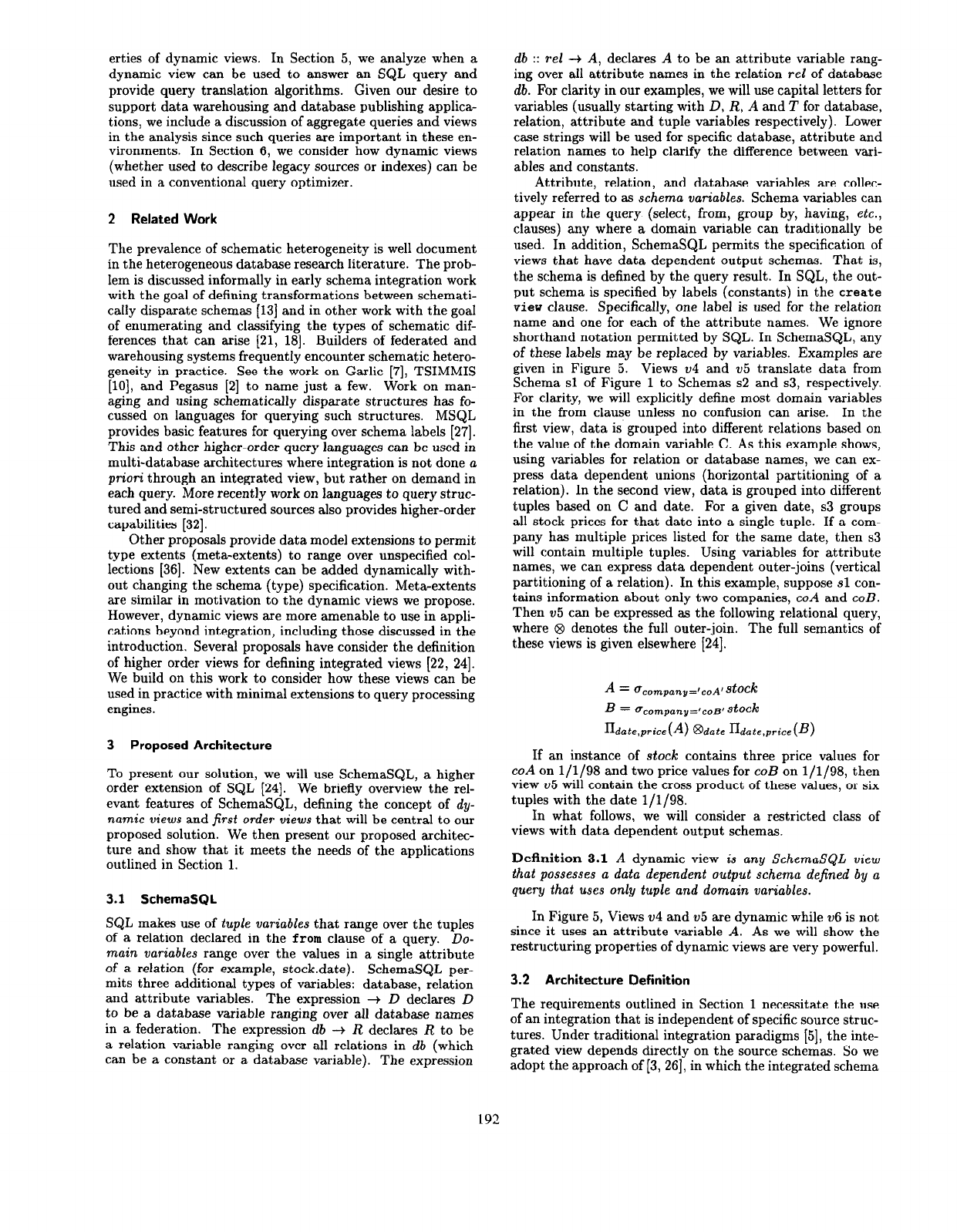
Using SQL, a single data independent view cannot be

constructed. Since SQL does not permit quantification over

relation or attribute names, any SQL view would have to in-

clude company names as constants. The view vl of Figure 2,

which translates data from Schema 92 to sl, illustrates this.

If the set of company names changes, the view definition

would need to be altered. To permit the specification of data

independent views, a language that permits quantification

over schema labels is needed. Many higher order languages

that include some form of quantification over schema con-

structs have been proposed. These include multi-database

languages [27], logics [ll, 231, algebras [33, 171, and object-

create view VI (co, date, price) as

( select ‘coA’, date, price

create view v2 (co, date, price) as

from coA

select R, T.date, T.price

union

from s2->R, R T

select ‘COB’, date, price

from COB

union

select ‘coC’, date, price

from coC

. . .

)

create view v3 (co, date, price) as

select A, T.date, T.A

from s3::stock->A, S3::stock T

where A # ‘date’

Figure 2: Example SQL and SchemaSQL views.

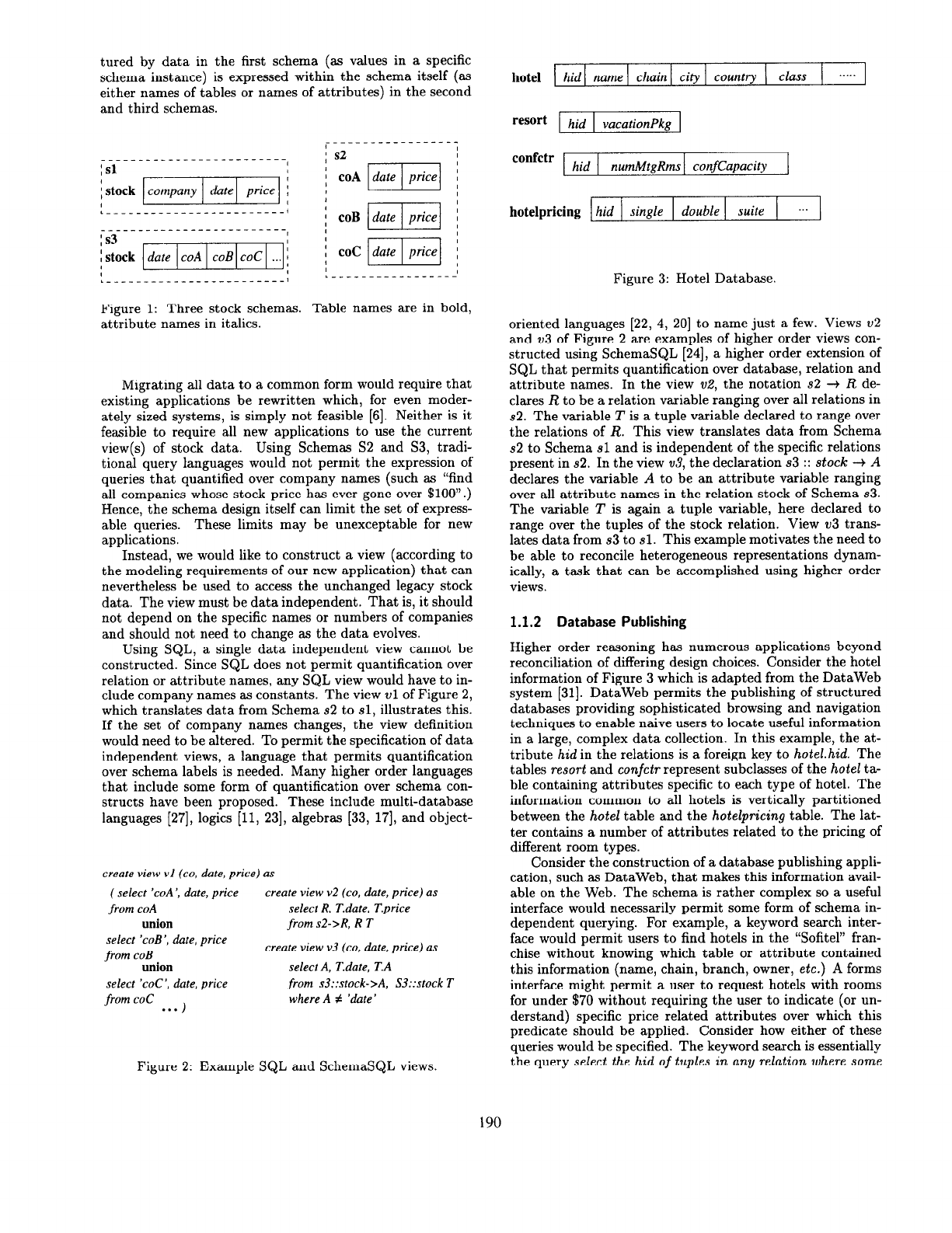
hotel

hid name chain city

country class

. . . . .

resort

hid vacationpkg

confctr

hid

numMtgRms confCapacity

hotelpricing

hid single double suite ...

Figure 3: Hotel Database.

oriented languages [22, 4, 201 to name just a few. Views v2

and v3 of Figure 2 are examples of higher order views con-

structed using SchemaSQL [24], a higher order extension of

SQL that permits quantification over database, relation and

attribute names. In the view v2, the notation 52 +

de-

clares

to be a relation variable ranging over all relations in

92. The variable

is a tuple variable declared to range over

the relations of

This view translates data from Schema

32 to Schema sl and is independent of the specific relations

present in 92. In the view v3, the declaration 93 ::

stock + A

declares the variable

to be an attribute variable ranging

over all attribute names in the relation stock of Schema 93.

The variable

is again a tuple variable, here declared to

range over the tuples of the stock relation. View v3 trans-

lates data from s3 to sl. This example motivates the need to

be able to reconcile heterogeneous representations dynam-

ically, a task that can be accomplished using higher order

views.

1.1.2 Database Publishing

Higher order reasoning has numerous applications beyond

reconciliation of differing design choices. Consider the hotel

information of Figure 3 which is adapted from the DataWeb

system [31]. DataWeb permits the publishing of structured

databases providing sophisticated browsing and navigation

techniques to enable naive users to locate useful information

in a large, complex data collection. In this example, the at-

tribute hid in the relations is a foreign key to

hoteLhid.

The

tables

resort

and

confctr

represent subclasses of the hotel ta-

ble containing attributes specific to each type of hotel. The

information common to all hotels is vertically partitioned

between the

hotel

table and the

hotelpricing

table. The lat-

ter contains a number of attributes related to the pricing of

different room types.

Consider the construction of a database publishing appli-

cation, such as DataWeb, that makes this information avail-

able on the Web. The schema is rather complex so a useful

interface would necessarily permit some form of schema in-

dependent querying. For example, a keyword search inter-

face would permit users to find hotels in the “Sofitel” fran-

chise without knowing which table or attribute contained

this information (name, chain, branch, owner, etc.) A forms

interface might permit a user to request hotels with rooms

for under $70 without requiring the user to indicate (or un-

derstand) specific price related attributes over which this

predicate should be applied. Consider how either of these

queries would be specified. The keyword search is essentially

the query

select the

hid of tuples in any relation

where some

190

attribute

value contains ‘Sofitel”. The inexpensive query is

select

hid

from hotelpricing

where

any attribute value is less

than 70. Both of these queries are higher order. Although

the information in the hotel database does not contain any

schematic discrepancies, the ability to answer queries over

schema components could be used to support the schema

independent querying required in this environment.

Suppose the information of Figure 3 has been collected

in a data warehouse and consider a decision analysis appli-

cation on this information. Specifically, assume the applica-

tion will need to aggregate hotel information over different

dimensions presenting a tabular (or data cube style [14])

summary to a user. An example query would be to find the

number of hotels in each country of each class (including

subtotals for all classes and all countries). Using this infor-

mation, a user can “drill down” to specific data of interest

by refining the dimensions over which aggregation is done

(for example, viewing information aggregated by country,

then by city). The concept of data dimensions is central to

decision analysis applications. They provide the axes over

which data can be “sliced and diced”. In the first genera-

tion of decision analysis systems, the dimensions were fixed

[12]. Many recent systems permit the dynamic creation (of

a potentially large numbers) of new dimensions [31]. In our

hotel example, this means the addition of new hierarchies

over which hotels can be aggregated. Dimensions may be

represented by attributes or sets of attributes. An exten-

sible analysis system requires the ability to reason over (a

time varying) set of new dimensions. Specifically, it must be

possible to permit the user to specify predicates that can be

applied to any subset of dimensions.

1.1.3 Physical Data Independence

Indexing architectures often use views to describe index struc-

tures in order to permit the integration of new indexes (or

access methods) into a query optimizer [8, 371. Tsatalos et

al [37] have developed a robust indexing architecture that

makes use of restricted views containing only selection, pro-

jection and join operations. The views are used to describe

a wide array of advanced indexing techniques. However,

they point out that their techniques cannot be used to de-

scribe indexing over subclasses of a class. This is due to

the lack of support for unions and for schema independent

views. Consider the class

tickets

that contains information

about traffic violations issued by the highway patrol which

is adapted from [l]. The class

tickets

contains the attributes

tnum, lit, infr describing the ticket number, license number

and infraction code respectively. Information kept by each

jurisdiction (a state or region within a state) is kept in a

subclass whose name is the jurisdiction’s name. Each ju-

risdiction maintains information about tickets issued in its

boundaries and in addition attempts (although perhaps not

consistently) to maintain information about all tickets given

to people holding licenses issued within its region. The def-

inition of a Bf-tree index keyed on the ticket infraction is

given in Figure 4 using the notation from [37]. The index

is defined over all jurisdictions. In [37], indices must be de-

scribed using SQL views and as a result, the proposal cannot

express or use indices over data dependent collections of ta-

bles (or classes). For example, indices over all subclasses of a

class cannot be express [37]. Using higher order views, such

indices can be expressed. However, to make use of these new

indices in query processing, it must be possible to determine

whether a view (index) can be used in answering a query.

Furthermore, it must be possible to determine what portion

create index ticketlnfr as btree by

create view dui(lic, infr) as

given T. infr select Tl.lic, T2.infr

select R, T.tnum, T.lic ,from ->R, R Tl, R T2

,from ->R, R T

where Tl.lic = T2.lic

and Tl.infr = ‘dui’

and Tl.tnum <> T2.tnum

Figure 4: Traffic ticket database.

of a query the view (index) answers.

Using higher order views, a wide class of useful new in-

dexing structures can be expressed. For example, consider

the view

dui

of Figure 4 which can be used to describe an

index helpful in evaluating data fusion [l] style queries. A

data fusion query involves the self-join of a union of tables.

The view dui finds all infractions issued to anyone with one

or more ‘DUI’ infraction (driving under the influence of al-

cohol). This view may describe an index that materializes

this specific fusion query.

Similarly, schematically disparate views of the data can

be used to model an inverted index that might be used

to support the evaluation of keyword search queries over

a structured database. By incorporating such views into an

architecture for supporting physical data independence, the

query optimizer can reason about the use of these indexing

structures and their combined used with traditional access

methods.

1.2 Paper Overview

In this paper, we develop techniques such as those required

in the above examples for understanding and managing sche-

matic heterogeneity. Our examples point to several different

scenarios in which some form of schematic reasoning is re-

quired. Indeed, the examples make use of higher order views,

higher order queries and higher order indexes (schema inde-

pendent indexes). On the surface, these examples seem to

necessitate full support for a higher order query language

and view definition facility capable of describing logical and

physical (index) structures. Specifically, the examples point

to the need for a language that is powerful enough to recon-

cile schematic heterogeneity and to describe heterogeneous

data representations. Additionally, they point to the need

for techniques to automatically translate queries against the

view into queries against the legacy schema(s) and to opti-

mize these modified queries.

Such extensions to a complex query processing engine

can be prohibitively expensive. We therefore take a prag-

matic approach. We propose a solution in which all sche-

matic heterogeneity is reconciled by a limited form of higher

order views called dynamic

views.

In Section 2, we overview the contributions of this work

and place it in the context of related work on schematic het-

erogeneity. In Section 3, we overview the proposed solution.

While our solution does not provide full support for higher

order reasoning, we show that it is still powerful enough

to meet the needs of the diverse applications we have just

outlined. In Section 4, we discuss the restructuring prop-

191

erties of dynamic views. In Section 5, we analyze when a

dynamic view can be used to answer an SQL query and

provide query translation algorithms. Given our desire to

support data warehousing and database publishing applica-

tions, we include a discussion of aggregate queries and views

in the analysis since such queries are important in these en-

vironments. In Section 6, we consider how dynamic views

(whether used to describe legacy sources or indexes) can be

used in a conventional query optimizer.

2 Related Work

The prevalence of schematic heterogeneity is well document

in the heterogeneous database research literature. The prob-

lem is discussed informally in early schema integration work

with the goal of defining transformations between schemati-

cally disparate schemas [13] and in other work with the goal

of enumerating and classifying the types of schematic dif-

ferences that can arise 121, 181. Builders of federated and

warehousing systems frequently encounter schematic hetero-

geneity in practice. See the work on Garlic [7], TSIMMIS

[lo], and Pegasus [2] to name just a few. Work on man-

aging and using schematically disparate structures has fo-

cussed on languages for querying such structures. MSQL

provides basic features for querying over schema labels [27].

This and other higher-order query languages can be used in

multi-database architectures where integration is not done a

priori through an integrated view, but rather on demand in

each query. More recently work on languages to query struc-

tured and semi-structured sources also provides higher-order

capabilities [32].

Other proposals provide data model extensions to permit

type extents (meta-extents) to range over unspecified col-

lections [36]. New extents can be added dynamically with-

out changing the schema (type) specification. Meta-extents

are similar in motivation to the dynamic views we propose.

However, dynamic views are more amenable to use in appli-

cations beyond integration, including those discussed in the

introduction. Several proposals have consider the definition

of higher order views for defining integrated views (22, 241.

We build on this work to consider how these views can be

used in practice with minimal extensions to query processing

engines.

3 Proposed Architecture

To present our solution, we will use SchemaSQL, a higher

order extension of SQL [24]. We briefly overview the rel-

evant features of SchemaSQL, defining the concept of dy-

namic views and

first

order views that will be central to our

proposed solution. We then present our proposed architec-

ture and show that it meets the needs of the applications

outlined in Section 1.

3.1 SchemaSQL

SQL makes use of tuple variables that range over the tuples

of a relation declared in the from clause of a query. Do-

main variables range over the values in a single attribute

of a relation (for example, stock.date). SchemaSQL per-

mits three additional types of variables: database, relation

and attribute variables. The expression + D declares D

to be a database variable ranging over all database names

in a federation. The expression db -+ R declares R to be

a relation variable ranging over all relations in db (which

can be a constant or a database variable). The expression

db :: rel -+ A, declares A to be an attribute variable rang-

ing over all attribute names in the relation rel of database

db. For clarity in our examples, we will use capital letters for

variables (usually starting with D, R, A and 2’ for database,

relation, attribute and tuple variables respectively). Lower

case strings will be used for specific database, attribute and

relation names to help clarify the difference between vari-

ables and constants.

Attribute, relation, and database variables are collec-

tively referred to as schema variables. Schema variables can

appear in the query (select, from, group by, having, etc.,

clauses) any where a domain variable can traditionally be

used. In addition, SchemaSQL permits the specification of

views that have data dependent output schemas. That is,

the schema is defined by the query result. In SQL, the out-

put schema is specified by labels (constants) in the create

view clause. Specifically, one label is used for the relation

name and one for each of the attribute names. We ignore

shorthand notation permitted by SQL. In SchemaSQL, any

of these labels may be replaced by variables. Examples are

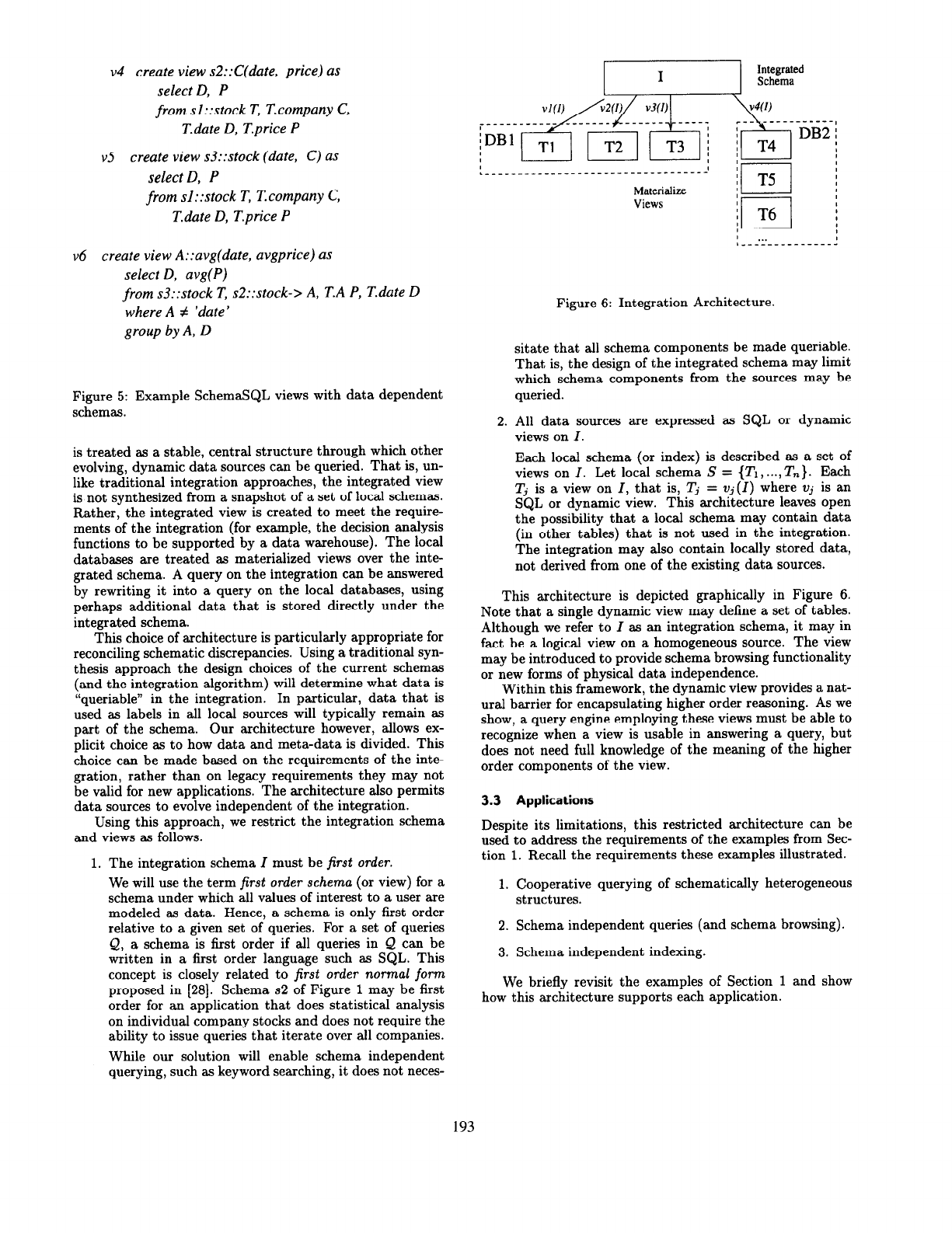
given in Figure 5. Views v4 and v5 translate data from

Schema sl of Figure 1 to Schema-s s2 and s3, respectively.

For clarity, we will explicitly define most domain variables

in the from clause unless no confusion can arise.

In the

first view, data is grouped into different relations based on

the value of the domain variable C. As this example shows,

using variables for relation or database names, we can ex-

press data dependent unions (horizontal partitioning of a

relation). In the second view, data is grouped into different

tuples based on C and date. For a given date, s3 groups

all stock prices for that date into a single tuple. If a com-

pany has multiple prices listed for the same date, then s3

will contain multiple tuples. Using variables for attribute

names, we can express data dependent outer-joins (vertical

partitioning of a relation). In this example, suppose sl con-

tains information about only two companies, coA and COB.

Then v5 can be expressed as the following relational query,

where @I denotes the full outer-join. The full semantics of

these views is given elsewhere [24].

~company=‘coA’~toC~

B = ucompany=~co~~ stock

date,price(A) @date ndate,price@)

If an instance of stock contains three price values for

coA on l/1/98 and two price values for COB on l/1/98, then

view v5 will contain the cross product of these values, or six

tuples with the date l/1/98.

In what follows, we will consider a restricted class of

views with data dependent output schemas.

Definition 3.1 A dynamic view is any SchemaSQL view

that possesses a data dependent output schema defined by a

query that uses only tuple and domain variables.

In Figure 5, Views v4 and v5 are dynamic while v6 is not

since it uses an attribute variable A. As we will show the

restructuring properties of dynamic views are very powerful.

3.2 Architecture Definition

The requirements outlined in Section 1 necessitate the use

of an integration that is independent of specific source struc-

tures. Under traditional integration paradigms [5], the inte-

grated view depends directly on the source schemas. So we

adopt the approach of [3,26], in which the integrated schema

192

v4 create view s2::C(date, price) as

select D, P

from sl::stock T, T.company C,

T.date D, T.price P

v.5

create view s3::stock (date, C) as

select D, P

from sl::stock T, T.company C,

T.date D, T.price P

v6 create view A::avg(date, avgprice) as

select D, avg(P)

from s3::stock T, s2::stock-> A, T.A P, T.date D

where A # ‘date’

group by A, D

Figure 5: Example SchemaSQL views with data dependent

schemas.

is treated as a stable, central structure through which other

evolving, dynamic data sources can be queried. That is, un-

like traditional integration approaches, the integrated view

is not synthesized from a snapshot of a set of local schemas.

Rather, the integrated view is created to meet the require-

ments of the integration (for example, the decision analysis

functions to be supported by a data warehouse). The local

databases are treated as materialized views over the inte-

grated schema. A query on the integration can be answered

by rewriting it into a query on the local databases, using

perhaps additional data that is stored directly under the

integrated schema.

This choice of architecture is particularly appropriate for

reconciling schematic discrepancies. Using a traditional syn-

thesis approach the design choices of the current schemas

(and the integration algorithm) will determine what data is

“queriable” in the integration. In particular, data that is

used as labels in all local sources will typically remain as

part of the schema. Our architecture however, allows ex-

plicit choice as to how data and meta-data is divided. This

choice can be made based on the requirements of the inte-

gration, rather than on legacy requirements they may not

be valid for new applications. The architecture also permits

data sources to evolve independent of the integration.

Using this approach, we restrict the integration schema

and views as follows.

1. The integration schema I must be first order.

We will use the term first order schema (or view) for a

schema under which all values of interest to a user are

modeled as data. Hence, a schema is only first order

relative to a given set of queries. For a set of queries

&, a schema is first order if all queries in & can be

written in a first order language such as SQL. This

concept is closely related to first order normal form

proposed in [28]. Schema s2 of Figure 1 may be first

order for an application that does statistical analysis

on individual company stocks and does not require the

ability to issue queries that iterate over all companies.

While our solution will enable schema independent

querying, such as keyword searching, it does not neces-

Materialize

Views

Figure 6: Integration Architecture.

sitate that all schema components be made queriable.

That is, the design of the integrated schema may limit

which schema components from the sources may be

queried.

All data sources are expressed as SQL or dynamic

views on

Each local schema (or index) is described as a set of

views on I. Let local schema S = {Ti, . . . .

T,,}.

Each

is a view on

that is,

Tj = vj(I)

where vj is an

SQL or dynamic view. This architecture leaves open

the possibility that a local schema may contain data

(in other tables) that is not used in the integration.

The integration may also contain locally stored data,

not derived from one of the existing data sources.

This architecture is depicted graphically in Figure 6.

Note that a single dynamic view may define a set of tables.

Although we refer to I as an integration schema, it may in

fact be a logical view on a homogeneous source. The view

may be introduced to provide schema browsing functionality

or new forms of physical data independence.

Within this framework, the dynamic view provides a nat-

ural barrier for encapsulating higher order reasoning. As we

show, a query engine employing these views must be able to

recognize when a view is usable in answering a query, but

does not need full knowledge of the meaning of the higher

order components of the view.

3.3 Applications

Despite its limitations, this restricted architecture can be

used to address the requirements of the examples from Sec-

tion 1. Recall the requirements these examples illustrated.

1. Cooperative querying of schematically heterogeneous

structures.

2. Schema independent queries (and schema browsing).

3. Schema independent indexing.

We briefly revisit the examples of Section 1 and show

how this architecture supports each application.

193

hprice

hid rmtype

price

create view hotelpricing(hid, R) as

select H, P

from hprice T, T.hid H, T.rmtype R, T.price P

select H

from hprice T, T.price P, T.hid H

where P < 70

Figure 7: Schema independent querying of hotelpricing.

Legacy System Integration

The Schema sl can be used as

the Integration I. All three schemas can then be represented

as dynamic views on I. The mapping from I to sl is the

identity map, and views v4 and v5 of Figure 5 provide the

definitions for s2 and 93. Queries posed on the integration

must be translated to queries on the legacy schemas (mate-

rialized views). To do this, an algorithm for translating any

SQL query into an SQL or SchemaSQL query on the un-

derlying views is required. This algorithm will permit the

answering of queries on the integration using data stored

under the legacy sources.

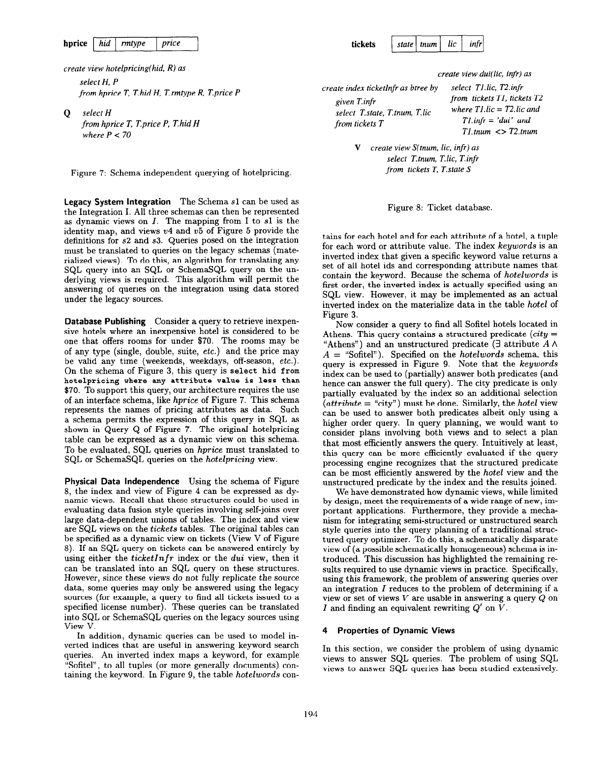
Database Publishing

Consider a query to retrieve inexpen-

sive hotels where an inexpensive hotel is considered to be

one that offers rooms for under $70. The rooms may be

of any type (single, double, suite, etc.) and the price may

be valid any time (weekends, weekdays, off-season, etc.).

On the schema of Figure 3, this query is select hid from

hotelpricing where any attribute value is less than

$70. To support this query, our architecture requires the use

of an interface schema, like hprice of Figure 7. This schema

represents the names of pricing attributes as data. Such

a schema permits the expression of this query in SQL as

shown in Query Q of Figure 7. The original hotelpricing

table can be expressed as a dynamic view on this schema.

To be evaluated, SQL queries on hprice must translated to

SQL or SchemaSQL queries on the

hotelpricing

view.

Physical Data Independence

Using the schema of Figure

8, the index and view of Figure 4 can be expressed as dy-

namic views. Recall that these structures could be used in

evaluating data fusion style queries involving self-joins over

large data-dependent unions of tables. The index and view

axe

SQL views on the

tickets

tables. The original tables can

be specified as a dynamic view on tickets (View V of Figure

8). If an SQL query on tickets can be answered entirely by

using either the

ticketInfr

index or the dui view, then it

can be translated into an SQL query on these structures.

However, since these views do not fully replicate the source

data, some queries may only be answered using the legacy

sources (for example, a query to find all tickets issued to a

specified license number). These queries can be translated

into SQL or SchemaSQL queries on the legacy sources using

View V.

In addition, dynamic queries can be used to model in-

verted indices that are useful in answering keyword search

queries. An inverted index maps a keyword, for example

“Sofitel”, to all tuples (or more generally documents) con-

taining the keyword. In Figure 9, the table

hotelwords

con-

tickets

state tnum lit infr

create view dui(lic, infr) as

create index ticketlnfr as btree by

select Tl.lic, T2.infr

given T.infr

from tickets TI, tickets T2

select T.state, T.tnum, T.lic

where Tl.lic = T2.lic and

from tickets T

Tl.infr = ‘dui’ and

Tl.tnum <> T2.tnum

V create view S(tnum, lit. infr) as

select T.tnum, T.lic, T.infr

from tickets T, T.state S

Figure 8: Ticket database.

tains for each hotel and for each attribute of a hotel, a tuple

for each word or attribute value. The index

keywords

is an

inverted index that given a specific keyword value returns a

set of all hotel ids and corresponding attribute names that

contain the keyword. Because the schema of

hotelwords

first order, the inverted index is actually specified using an

SQL view. However, it may be implemented as an actual

inverted index on the materialize data in the table

hotel

Figure 3.

Now consider a query to find all Sofitel hotels located in

Athens. This query contains a structured predicate

(city =

“Athens”) and an unstructured predicate (3 attribute

A A

= “Sofitel”). Specified on the

hotelwords

schema, this

query is expressed in Figure 9. Note that the

keywords

index can be used to (partially) answer both predicates (and

hence can answer the full query). The city predicate is only

partially evaluated by the index so an additional selection

(attribute

= “city”) must be done. Similarly, the

hotel

view

can be used to answer both predicates albeit only using a

higher order query. In query planning, we would want to

consider plans involving both views and to select a plan

that most efficiently answers the query. Intuitively at least,

this query can be more efficiently evaluated if the query

processing engine recognizes that the structured predicate

can be most efficiently answered by the

hotel

view and the

unstructyred predicate by the index and the results joined.

We have demonstrated how dynamic views, while limited

by design, meet the requirements of a wide range of new, im-

portant applications. Furthermore, they provide a mecha-

nism for integrating semi-structured or unstructured search

style queries into the query planning of a traditional struc-

tured query optimizer. To do this, a schematically disparate

view of (a possible schematically homogeneous) schema is in-

troduced. This discussion has highlighted the remaining re-

sults required to use dynamic views in practice. Specifically,

using this framework, the problem of answering queries over

an integration I reduces to the problem of determining if a

view or set of views

are usable in answering a query Q on

and finding an equivalent rewriting Q’ on

4 Properties of Dynamic Views

In this section, we consider the problem of using dynamic

views to answer SQL queries. The problem of using SQL

views to answer SQL queries has been studied extensively.

194

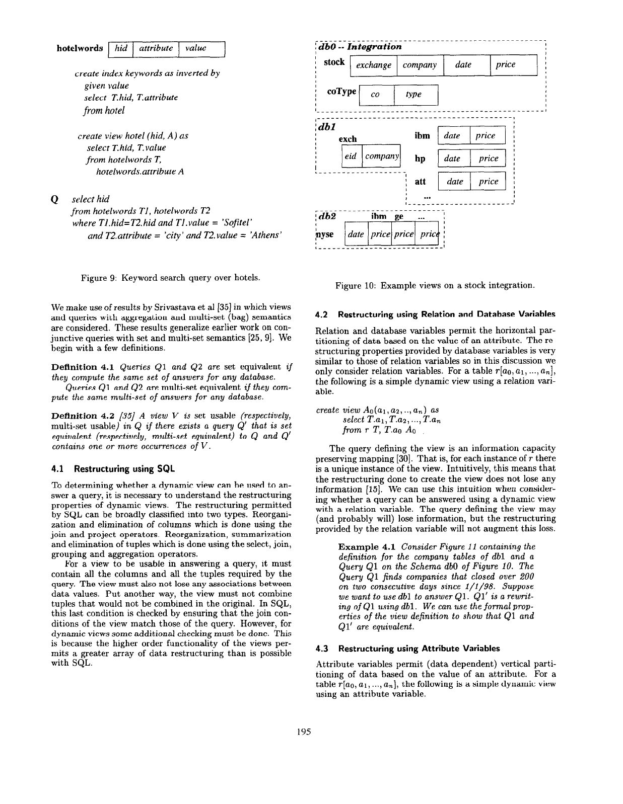
hotelwords hid attribute value

create index keywords as inverted by

given value

select T.hid, T.attribute

from hotel

create view hotel (hid, A) as

select T.hid, T.value

from hotelwords T,

hotelwords.attribute A

select hid

from hotelwords TI, hotelwords T2

where Tl.hid=T2.hid and Tl.value = ‘Sofitel’

and T2.attribute = ‘city’ and 72.value = ‘Athens’

Figure 9: Keyword search query over hotels.

We make use of results by Srivastava et al [35] in which views

and queries with aggregation and multi-set (bag) semantics

are considered. These results generalize earlier work on con-

junctive queries with set and multi-set semantics [25, 91. We

begin with a few definitions.

Definition 4.1 Queries Ql

and

are

set equivalent 2f

they compute the same set of answers

for

any database.

Queries Ql and Q2 are multi-set equivalent if they com-

pute the same multi-set of answers

for

any database.

Definition 4.2 1351

view

is set usable

(respectively,

multi-set usable) in Q if there exists a query Q’ that is set

equivalent (respectively, multi-set equivalent) to Q and Q’

contains one

more occurrences of V.

4.1 Restructuring using SQL

To determining whether a dynamic view can be used to an-

swer a query, it is necessary to understand the restructuring

properties of dynamic views. The restructuring permitted

by SQL can be broadly classified into two types. Reorgani-

zation and elimination of columns which is done using the

join and project operators. Reorganization, summarization

and elimination of tuples which is done

using

the select, join,

grouping and aggregation operators.

For a view to be usable in answering a query, it must

contain all the columns and all the tuples required by the

query. The view must also not lose any associations between

data values. Put another way, the view must not combine

tuples that would not be combined in the original. In SQL,

this last condition is checked by ensuring that the join con-

ditions of the view match those of the query. However, for

dynamic views some additional checking must be done. This

is because the higher order functionality of the views per-

mits a greater array of data restructuring than is possible

with SQL.

i db0 -- Integration

: stock

exchange

company

date

price

i dbl

‘--------‘--;-‘-------------

; db2

lbm ge . . . I

r I I I I ’

F [date 1 price1 price1 pric{ i

I_________________-_--------

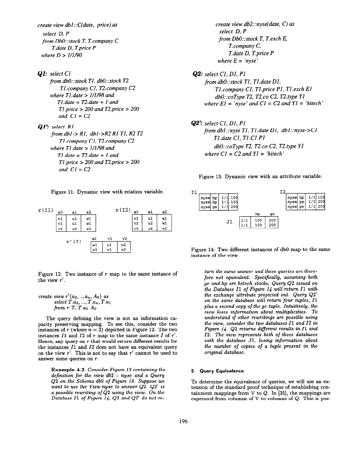
Figure 10: Example views on a stock integration.

4.2 Restructuring using Relation and Database Variables

Relation and database variables permit the horizontal par-

titioning of data baaed on the value of an attribute. The re-

structuring properties provided by database variables is very

similar to those of relation variables so in this discussion we

only consider relation variables. For a table

r[m,al, . . . . a,],

the following is a simple dynamic view using a relation var-

able.

create view Ao(al, a~, .., a,) as

select T.al, T.ag, . . . . T.a,

from

T, T.ao

The query defining the view is an information capacity

preserving mapping [30]. That is, for each instance of

there

is a unique instance of the view. Intuitively, this means that

the restructuring done to create the view does not lose any

information [15]. We can use this intuition when consider-

ing whether a query can be answered using a dynamic view

with a relation variable. The query defining the view may

(and probably will) lose information, but the restructuring

provided by the relation variable will not augment this loss.

Example 4.1

Consider Figure 11 containing the

definition

for

the company tables of

dbl and a

Query Ql on the Schema db0 of Figure 10. The

Query Ql finds companies that closed over 200

two

consecutive days since l/1/98. Suppose

we want to use dbl to answer Ql. Ql’ is a rewrit-

ing of Ql using dbl. We can use the formal

prop-

erties of the view definition to show that Ql and

Ql’ are equivalent.

4.3 Restructuring using Attribute Variables

Attribute variables permit (data dependent) vertical parti-

tioning of data based on the value of an attribute. For a

table r[ao, al, . . . . a,], the following is a simple dynamic view

using an attribute variable.

195

create view dbl::C(date, price) as

select D, P

from DbO::stock T, T.company C

T.date D, T.price P

where D > l/1/90

Ql:

select Cl

from dbO::stock TI, dbO::stock T2

Tl.company Cl, lL?company C2

where Tl.date > l/1/98 and

Tl.date = T2.a’ate + 1 and

Tl.price > 200 and T2.price > 200

and Cl = C2

Ql':

select RI

from dbl-> RI, dbl->R2 Rl TI, R2 T2

Tl.company Cl, T2.company C2

where Tl.date > l/U98 and

Tl.date = T2.date + 1 and

Tl.price > 200 and T2.price > 200

and Cl = C2

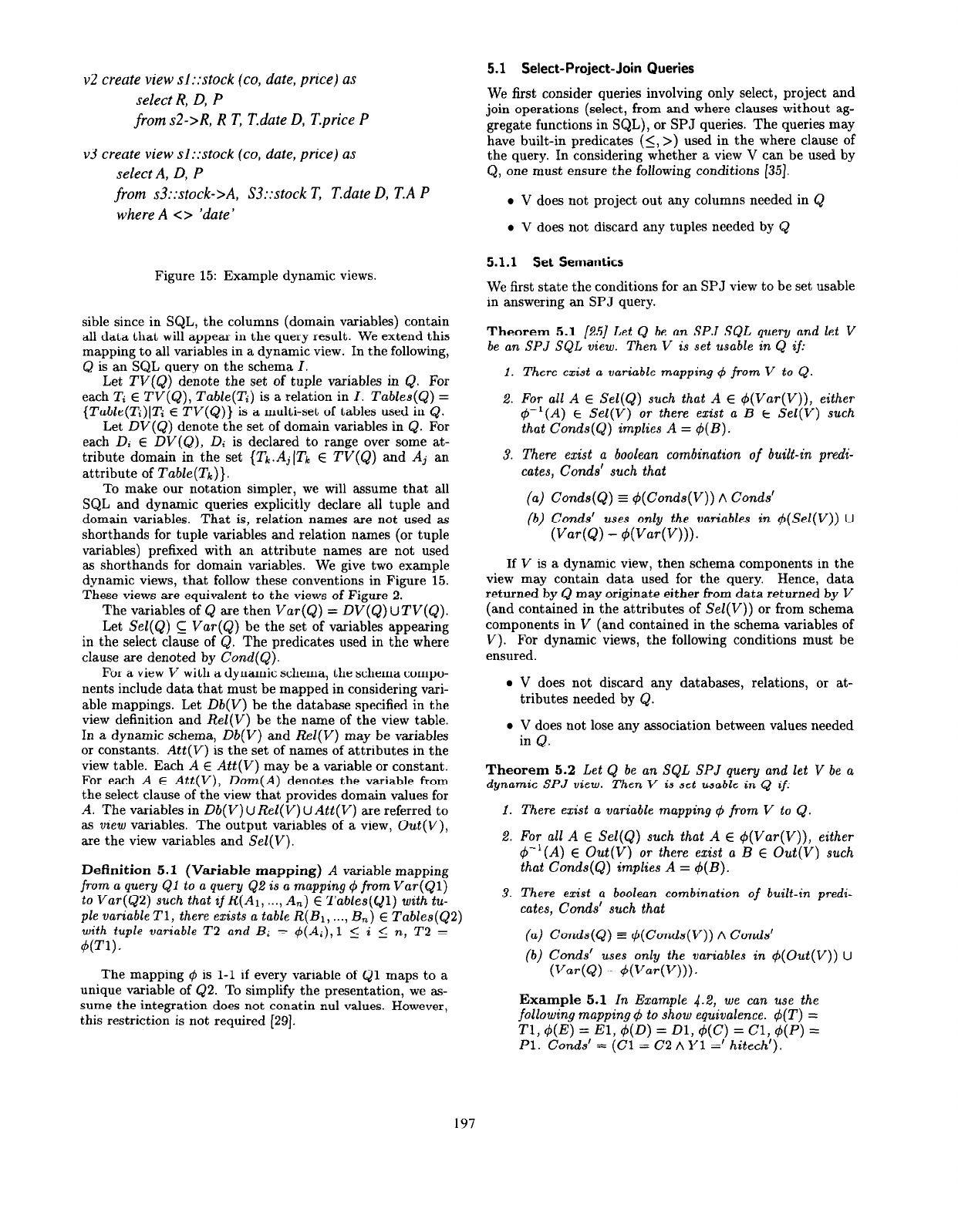
Figure 11: Dynamic view with relation variable.

r(I1) a0 al a2 r (12)

mi WI

r’(1) pT$-Tg]

Figure 12: Two instance of r map to the same instance of

the view

T'.

create view r’(aa, .., a,, Ao) as

select T.az, . . . . T.a,, T.al

from

T, T.ao Ao

The query defining the view is not an information ca-

pacity preserving mapping. To see this, consider the two

instances of r (where n = 2) depicted in Figure 12. The two

instances Zl and 12 of T map to the same instance Z of r’.

Hence, any query on T that would return different results for

the instances Zl and 12 does not have an equivalent query

on the view

T'.

This is not to say that

T’

cannot be used to

answer some queries on T.

Example 4.2

Consider Figure 13 containing the

definition

for

the view db2 :: nyse and a Query

Q2 on the Schema db0 of Figure 10. Suppose we

want to use the View nyse to answer Q2. Q2’ is

a possible rewriting of Q2 using the view. On the

Database Zl of Figure 14, Q2 and Q2’ do not re-

create view db2::nyse(date, C) as

select D, P

from DbO::stock T, T.exch E,

T.company C,

T.date D, T.price P

where E = ‘nyse’

Q2: select Cl, DI, PI

from dbO::stock TI, Tl.date Dl,

Tl.company Cl, Tl.price PI, Tl.exch El

dbO::coType T2, T2.co C2, T2.type Yl

where El = ‘nyse’ and Cl = C2 and YI = ‘hitech’

Q2’: select Cl, Dl, PI

from dbl::nyse Tl, Tl.date Dl, dbl::nyse->Cl

Tl.date Cl, Tl.Cl PI

dbO::coType T2, T2.co C2, T2.type Yl

where Cl = C2 and YI = ‘hitech’

Figure 13: Dynamic view with an attribute variable.

Figure 14: Two different instances of db0 map to the same

instance of the view.

turn the same answer and these queries

are

there-

fore not equivalent. Specifically, assuming both

ge and hp are hitech stocks,

Query Q2

issued on

the Database Zl of Figure 14 will return Zl with

the exchange attribute projected out. Query 92’

on the same database will return four tuples, Zl

plus a second copy of the ge tuple. Intuitively, the

view loses information about multiplicities. To

understand if other rewritings are possible using

the view, consider the two databases Zl and 12 in

Figure 14. Q2 returns different results in Zl and

12. The view represents both of these databases

with the database Jl, losing information about

the number of copies of a tuple present in the

original database.

5 Query Equivalence

To determine the equivalence of queries, we will use an

ex-

tension of the standard proof technique of establishing con-

tainment mappings from V to Q. In [35], the mappings are

expressed from columns of V to columns of Q. This is

pas-

196

v2 create view sl::stock (co, date, price) as

select R, D, P

from s2->R, R T, T.date D, T.price P

v3 create view sl::stock (co, date, price) as

select A, D, P

from s3::stock->A, S3::stock T, T.date D, T.A P

where A c> ‘date’

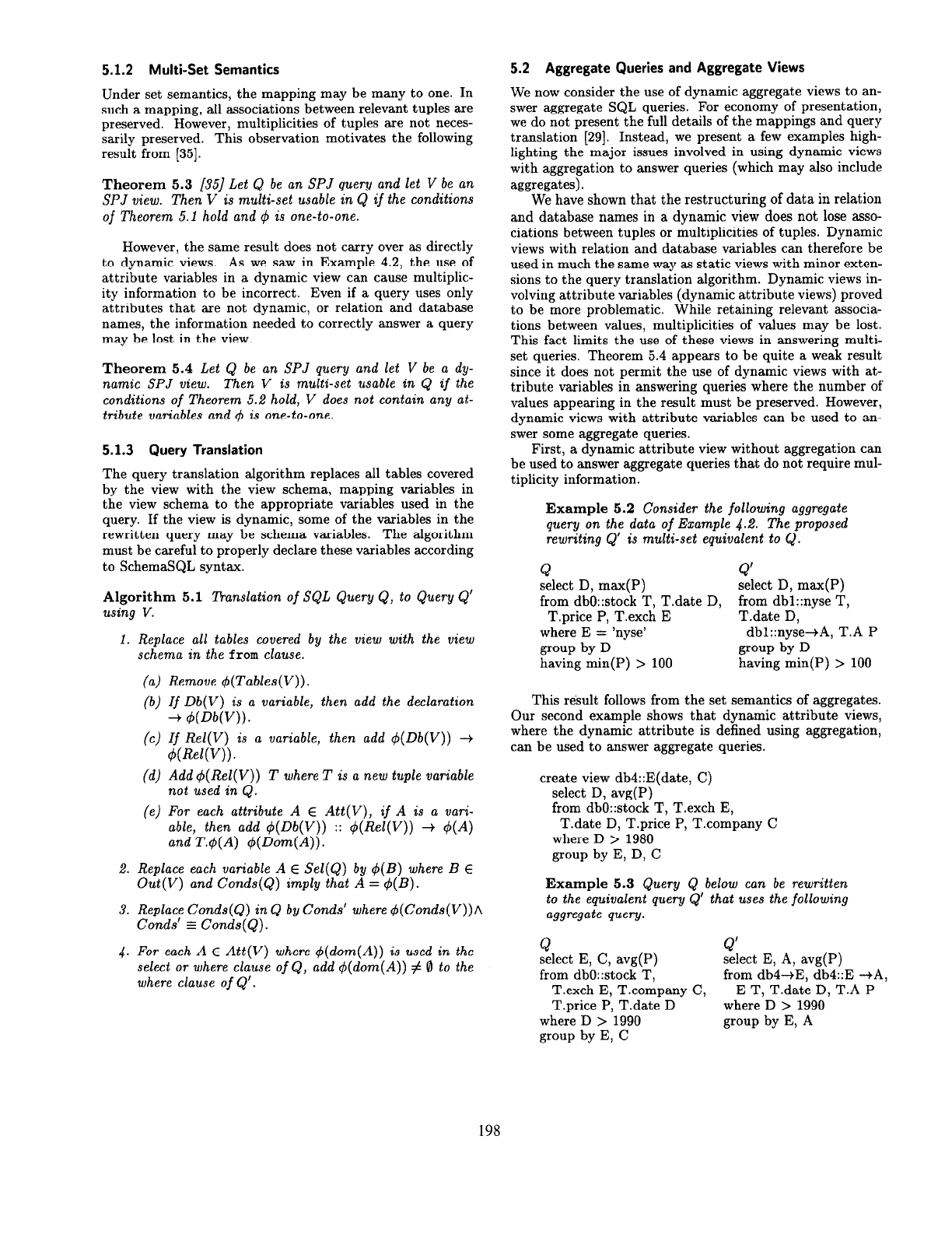
Figure 15: Example dynamic views.

sible since in SQL, the columns (domain variables) contain

all data that will appear in the query result. We extend this

mapping to all variables in a dynamic view. In the following,

Q is an SQL query on the schema I.

Let TV(Q) denote the set of tuple variables in Q. For

each T; E TV(Q), Table(Ti) is a relation in I. Tables(Q) =

{Table(T; E TV(Q)} is a multi-set of tables used in Q.

Let DV(Q) denote the set of domain variables in Q. For

each Di E DV(Q), Di is declared to range over some at-

tribute domain in the set {Th.Aj(Tk E TV(Q) and Aj an

attribute of Table(Tk)}.

To make our notation simpler, we will assume that all

SQL and dynamic queries explicitly declare all tuple and

domain variables. That is, relation names are not used as

shorthands for tuple variables and relation names (or tuple

variables) prefixed with an attribute names are not used

as shorthands for domain variables. We give two example

dynamic views, that follow these conventions in Figure 15.

These views are equivalent to the views of Figure 2.

The variables of Q are then Var(Q) = DV(Q) UTV(Q).

Let Sel(Q) E Var(Q) be the set of variables appearing

in the select clause of Q. The predicates used in the where

clause are denoted by Cond(Q).

For a view V with a dynamic schema, the schema compo-

nents include data that must be mapped in considering vari-

able mappings. Let Db(V) be the database specified in the

view definition and Rel(V) be the name of the view table.

In a dynamic schema, Db(V) and Rel(V) may be variables

or constants. Att(V) is the set of names of attributes in the

view table. Each A E Att(V) may be a variable or constant.

For each A E AH(V), Dam(A) denotes the variable from

the select clause of the view that provides domain values for

A. The variables in Db(V) UReZ(V) UAtt(V) axe referred to

as view variables. The output variables of a view, Out(V),

are the view variables and Sel(V).

Definition 5.1 (Variable mapping)

A variable mapping

from a query Ql to a query 9.2 is a mapping 4 from Var(QI)

to Var(Q2) such that if R(A1, . . . . An) E Tables(Q1) with tu-

pie variable Tl, there exists a table R(B1, . . . . B,) E Tables(Q2)

with tuple variable T2 and Bi = +(Ai), 1 < i 5 n, T2 =

do.

The mapping 4 is l-l if every variable of Ql maps to a

unique variable of Q2. To simplify the presentation, we as-

sume the integration does not conatin nul values. However,

this restriction is not required [29].

5.1 Select-Project-Join Queries

We first consider queries involving only select, project and

join operations (select, from and where clauses without ag-

gregate functions in SQL), or SPJ queries. The queries may

have built-in predicates (5, >) used in the where clause of

the query. In considering whether a view V can be used by

Q, one must ensure the following conditions [35].

V does not project out any columns needed in Q

V does not discard any tuples needed by Q

5.1.1 Set Semantics

We first state the conditions for an SPJ view to be set usable

in answering an SPJ query.

Theorem 5.1 [25]

Let Q be an SPJ SQL query and let V

be an SPJ SQL view. Then V is set usable in Q if:

There exist a variable mapping 4 from V to Q.

FOT all A E Sel(Q) such that A E $(Var(V)), either

$-‘(A) E Sel(V)

there exist a B E Sel(V) such

dhat Conds(Q) implies A = d(B).

There

exist a boolean combination of built-in predi-

cates, Conds’ such that

(a) Conds(Q) E +(Conds(V)) A Conds’

(b) Conds’ uses only the variables in q5(Sel(V)) U

(Var(&) - d(Var(V))).

If V is a dynamic view, then schema components in the

view may contain data used for the query. Hence, data

returned by Q may originate either from data returned by V

(and contained in the attributes of Sel(V)) or from schema

components in V (and contained in the schema variables of

V). For dynamic views, the following conditions must be

ensured.

V does not discard any databases, relations, or at-

tributes needed by Q.

V does not lose any association between values needed

in Q.

Theorem 5.2

Let Q be an SQL SPJ query and let V be a

dynamic SPJ view. Then V is set usable in Q if:

1. There exist a variable mapping 4 from V to Q.

2. FOT all A E Sel(Q) such that A E 4(Var(V)), either

4-‘(A) E Out(V)

there exist a

B E Out(V)

such

that Conds(Q) implies A = 4(B).

3. There exist a boolean combination of built-in predi-

cates, Conds’ such that

(a) Conds(Q) E 4(Conds(V)) A Conds’

(b) Conds’ uses only the variables in +(Out(V)) U

(Var(&) - 4(Var(v))).

Example 5.1

In Example 4.2, we can use the

following mapping 4 to show equivalence. d(T) =

Tl, 4(E) = El, 4(D) = Dl, 4(C) = Cl, d(P) =

Pl. Conds’ = (Cl = C2 A Y 1 =’ hitech’).

197

5.1.2 Multi-Set Semantics

Under set semantics, the mapping may be many to one. In

such a mapping, all associations between relevant tuples are

preserved. However, multiplicities of tuples are not neces-

sarily preserved. This observation motivates the following

result from [35].

Theorem 5.3 [35]

Let Q be an SPJ query and let V be an

SPJ view. Then V is multi-set usable in Q if the conditions

of Theorem 5.1 hold and 4 is one-to-one.

However, the same result does not carry over as directly

to dynamic views. As we saw in Example 4.2, the use of

attribute variables in a dynamic view can cause multiplic-

ity information to be incorrect. Even if a query uses only

attributes that are not dynamic, or relation and database

names, the information needed to correctly answer a query

may be lost in the view.

Theorem 5.4

Let Q be an SPJ query and let V be a dy-

namic SPJ view. Then V is multi-set usable in Q if the

conditions

Theorem 5.2 hold, V does not contain any at-

tribute variables and I$ is one-to-one.

5.1.3 Query Translation

The query translation algorithm replaces all tables covered

by the view with the view schema, mapping variables in

the view schema to the appropriate variables used in the

query. If the view is dynamic, some of the variables in the

rewritten query may be schema variables. The algorithm

must be careful to properly declare these variables according

to SchemaSQL syntax.

fgrchm 5.1

Translation

SQL Query Q, to Query Q’

Replace all tables covered by the view with the view

schema in the from clause.

(b)

Remove $(Tables(V)).

If Db(V) is a variable, then add the declaration

+ WW’)).

Rel(V) is a variable, then add d(Db(V)) -+

d(ReW?).

Add d(Rel(V)) T where T is a new tuple variable

not used in Q.

For each attribute A E Att(V), if A is a vari-

able, then add 4(Db(V)) :: 4(ReZ(V)) + +(A)

and T&(A) 4(Dom(A)).

Replace each variable A E Sel(Q) by 4(B) where B E

Out(V) and Conds(Q) imply that A = d(B).

Replace Conds(Q) in Q by Conds’ where 4(Conds(V))r\

Conds’ s Conds( Q) .

For each A E Att(V) where #(dam(A)) is used in the

select or where clause

Q, add +(dom(A)) # 0 to the

where clause

Q’.

5.2 Aggregate Queries and Aggregate Views

We now consider the use of dynamic aggregate views to an-

swer aggregate SQL queries. For economy of presentation,

we do not present the full details of the mappings and query

translation [29]. Instead, we present a few examples high-

lighting the major issues involved in using dynamic views

with aggregation to answer queries (which may also include

aggregates).

We have shown that the restructuring of data in relation

and database names in a dynamic view does not lose asso-

ciations between tuples or multiplicities of tuples. Dynamic

views with relation and database variables can therefore be

used in much the same way as static views with minor exten-

sions to the query translation algorithm. Dynamic views in-

volving attribute variables (dynamic attribute views) proved

to be more problematic. While retaining relevant associa-

tions between values, multiplicities of values may be lost.

This fact limits the use of these views in answering multi-

set queries. Theorem 5.4 appears to be quite a weak result

since it does not permit the use of dynamic views with at-

tribute variables in answering queries where the number of

values appearing in the result must be preserved. However,

dynamic views with attribute variables can be used to an-

swer some aggregate queries.

First, a dynamic attribute view without aggregation can

be used to answer aggregate queries that do not require mul-

tiplicity information.

Example

5.2 Consider the following aggregate

query on the data

Example

4.2.

The proposed

rewriting Q’ is multi-set equivalent to Q.

Q’

select D, max(P) select D, max(P)

from dbO::stock T, T.date D, from dbl::nyse T,

T.price P, T.exch E T.date D,

where E = ‘nyse’

dbl::nyse+A, T.A P

group by D

having min(P) > 100 having min(P) > 100

This result follows from the set semantics of aggregates.

Our second example shows that dynamic attribute views,

where the dynamic attribute is defined using aggregation,

can be used to answer aggregate queries.

create view db4::E(date, C)

select D, avg(P)

from dbO::stock T, T.exch E,

T.date D, T.price P, T.company C

where D > 1980

group by E, D, C

Example 5.3

Query Q below can be rewritten

to the equivalent query Q’ that uses the following

aggregate query.

Q’

select E, C, avg(P)

select E, A, avg(P)

from dbO::stock T, from db4-+E, db4::E -+A,

T.exch E, T.company C, E T, T.date D, T.A P

T.price P, T.date D where D > 1990

where D > 1990 group by E, A

group by E, C

198

Integration with a Query Optimizer

The usability criteria and query translation algorithms of the

previous section permit the selection of views that can cor-

rectly be used to answer a query. However, they do not ad-

dress the issue of optimizing queries over a set of views. For

SPJ queries and views, this issue has been addressed [8, 371

by extending the common dynamic programming style op-

timizer [34] to consider plans using views. Two primary

extensions are necessary. First, in addition to access meth-

ods to base relation, the optimizer must consider the use

of views to build a query plan. These views may in turn

describe index structures. Second, it must be possible to

quickly determine what portion of a query a view answers

and whether a plan built from views and other access meth-

ods is a partial or complete answer to the query.

A conventional optimizer begins by finding execution

plans for single relations, then iteratively finds execution

plans for successively larger portions of a query. In the pres-

ence of materialized views or indices described by views, the

initial set of access plans is extended to include these views.

Chaudhuri et al [8] show how for SPJ views, a simple data

structure can be used to record the portion of the query an-

swered by the view. This is possible because an SPJ view

will replace (or answer) a set of tables and predicates in the

query and possibly add a new set of predicates (Conds’ from

the translation algorithm). Using only these sets (tables and

predicates answered by the view and new predicates added

as a result of the view), the optimizer can determine whether

a plan using a set of views is partial or complete. For par-

tial plans, the set of tables and predicates that remain to be

addressed can be computed.

We have shown that for dynamic SPJ views, the portion

of a query answered by a view can also be modeled in the

same way. That is, the query translation process involves

determining a set of tables and predicates from the query

that can be replaced by the view. A query optimizer can

therefore treat dynamic views as primitive access plans irre-

gardless of whether the view is implemented by an external

data source or by an internal index. The higher order prop-

erties of the view must be analyzed to determine if the view

is usable but additional analysis of this information is not

required by the optimizer. In particular, only the index or

external source needs to be able to execute the, possibly

higher order, plan.

Note that this form of integration with a query optimizer

permits correct use of dynamic views while requiring mini-

mal extensions to the optimizer.

7 Conclusions

The existence of schematic heterogeneity in legacy systems

is well document in the research literature. Many of the

more than thirty representations for a single data fact, enu-

merated by Kent result from some type of schematic hetero-

geneity [19]. Despite its prevalence, and despite the plethora

of work on enumerating and categorizing types of schematic

heterogeneity, no systematic study of how this schematically

heterogeneous structures can be used and queried in prac-

tice has been undertaken. We have provided a first step

in such a study. Specifically, we have analyzed the prop-

erties of restructuring transformations required to resolve

schematic discrepancies. Using this analysis we have showed

how higher order views can be used in answering queries on

schematically heterogeneous structures. We have showed

that our solution is powerful enough to meet the needs of

numerous applications drawn from the realms of data ware-

housing, decision support, database publishing and physical

data independence. The solutions allow access methods for

semi-structured and unstructured data to be incorporated

into the framework of structured query evaluation and op-

timization.

References

I31

[51

]71

191

PO1

[III

S. Abiteboul, H. Garcia-Molina, Y. Papakonstanti-

nou, and R. Yerneni. Fusion Queries over Internet

Databases. Technical Report unpublished manuscript,

Stanford University, 1997.

R. Ahmed, P. DeSmedt, W. Du, W. Kent, M. A.

Ketabchi, W. A. Litwin, A. Rafii, and M. C. Shan. The

Pegasus Heterogeneous Multidatabase System. IEEE

Computer, 24(12):19-27, December 1991.

Y. Arens, C. Y. Chee, C. N. Hsu, and C. A. Knoblock.

Retrieving and Integrating Data from Multiple Infor-

mation Sources. Intl. J. of Intelligent and

Cooperative

Info. Systems, 2(2):127-158, 1993.

T. Barsalou and D. Gangopadhyay. M(DM): An Open

Framework for Interoperation of Multimode1 Multi-

database Systems. In Proc. of the Int? Conf. on Data

Eng., pages 218-227, Tempe, AZ, February 1992.

C. Batini, M. Lenzerini, and S. B. Navathe. A Compar-

ative Analysis of Methodologies for Database Schema

Integration. ACM Computing Surveys, 18(4):323-364,

December 1986.

M. L. Brodie and M. Stonebraker. Migrating Legacy

Systems: Gateways, Interfaces, and the Incremental

Approach. Morgan Kaufmann Series in Data Mngmt.

Sys., Jim Gray, Ed. Morgan Kaufmann, 1995.

M. J. Carey, L. M. Haas, P. M. Schwarz, M. Arya,

W. F. Cody, R. Fagin, M. Flickner, A. W. Luniewski,

W. Niblack, D. Petkovic, J. Thomas, J. H. Williams,

and E. L. Wimmers. Towards Heterogeneous Multi-

media Information Systems: The Garlic Approach. In

Proc. of the Fifth Int’l IEEE Wksp. on Research Issues

in Data Eng. (RIDE-95): Distributed Object Mngmt.,

Taipei, Taiwan, March 1995.

S. Chaudhuri, R. Krishnamurthy, S. Potamianos, and

K. Shim. Optimizing Queries with Materialized Views.

In PTOC. of the Int’l Conf. on Data Eng., pages 190-200.

IEEE, 1995.

S. Chaudhuri and M. Y. Vardi. Optimization of Real

Conjunctive Queries. In Proc. of the ACM Symp. on

Principles of Database Systems (PODS), 1993.

S. Chawathe, H. Garcia-Molina, J. Hammer, K. Ire-

land, Y. Papakonstantinou, J. Ullman, and J. Widom.

The TSIMMIS Project: Integration of Heterogeneous

Information Sources. In Proc. of the 100th Anniver-

sary Meeting of the Information Processing Society of

Japan(IPSJ), pages 7-18, Tokyo, Japan, October 1994.

W. Chen, M. Kifer, and D. S. Warren. HiLog as a

Platform for Database Languages. In Int’l Workshop

on Database Programming Languages, pages 315-329,

Gleneden Beach, OR, June 1989.

199

[12] E.F Codd and S. B. Codd. Providing OLAP (On-line

Analytical Processing) to User-Analysts: An IT Man-

date. Technical report, E.F. Codd and Associates, 1994.

[13] U. Dayal and H. Y. Hwang. View Definition and Gen-

eralization for Database Integration in a Multidatabase

System. IEEE Trans. on

Software

Engineering, SE-

10(6):628-644, November 1984.

[14] J. Gary, A. Bosworth, A. Layman, and H. Pirahesh.

Data Cube: A Relational Aggregation Operator Gener-

alizing Group-By, Cross-Tab, and Sub-Totals. In Proc.

of the Int’l Conf. on Data Eng., pages 152-159, 1996.

[15] R. Hull. Relative Information Capacity of Simple Re-

lational Database Schemata. Society

for

Industrial and

Applied Mathematics (SIAM) Journal of Computing,

15(3):856-886, August 1986.

[16] R. Hull.

Managing Semantic Heterogeneity in

Databases: A Theoretical Perspective. In Proc. of

the ACM Symp. on Principles of Database Systems

(PODS), pages 51-61, 1997.

[17] D. Van Gucht J. Van den Bussche and G. Vossen. Re-

flective Programming in the Relational Algebra. In

Proc. of the ACM Symp. on Principles of Database Sys-

tems (PODS), pages 17-25, 1993.

[18] V. Kashyap and A. Sheth. Semantic and Schematic

Similarities between Database Objects: A Context-

based Approach. The Int? Journal on Very Large Data

Bases, 5(4):276-304, December 1996.

[19] W. Kent. The Many Forms of a Single Fact. In Proc. of

IEEE Int’l Computer Conf. (COMPCON), pages 438-

443, 1989.

[20] M. Kifer, W. Kim, and Y. Sagiv. Querying Object-

Oriented Databases. In ACM SIGMOD Int’l Conf. on

the Management of Data, pages 393-402, 1992.

[21] W. Kim and J. Seo. Classifying Schematic and Data

Heterogeneity in Multidatabase Systems. IEEE Com-

puter,

24(12):12-18, December 1991.

[22] R. Krishnamurthy, W. Litwin, and W. Kent. Language

Features for Interoperability of Databases with Sche-

matic Discrepancies. In ACM SIGMOD Int’l Conf. on

the Management of Data, pages 40-49, 1991.

123) L. Lakshmanam, F. Sadri, and I. N. Subramanian.

On the Logical Foundations of Schema Integration and

Evolution in Heterogeneous Database Systems. In Proc.

of the Int?. Conf. on Deductive and Object-Oriented

Databases, 1993.

[24] L. Lakshmanam, F. Sadri, and I. N. Subramanian.

SchemaSQL - A Language for Interoperability in Re-

lational Multi-database Systems. In Proc. of the Int’l

Conf. on Very Large Data Bases (VLDB), Bombay, In-

dia, 1996.

[25] A. Y. Levy, A. 0. Mendelzon, Y. Sagiv, and D. Sri-

vastava. Answering Queries Using Views. In Proc.

of the ACM Symp. on Principles of Database Systems

(PODS), San Jose, CA, May 1995.

[26] A. Y. Levy, A. Rajaraman, and J. J. Ordille. Querying

Heterogeneous Information Sources Using Source De-

scriptions. In PTOC. of the Int’l Conf. on Very Large

Data Bases (VLDB), pages 251-262, Bombay, India,

1996.

[27] W. Litwin and A. Abdellatif. Multidatabase Interoper-

ability. IEEE Computer, 19(12):10-18, December 1986.

[28] W. Litwin, M. Ketabchi, and R. Krishnamurthy. First

Order Normal Form for Relational Databases and Mul-

tidatabases. SIGMOD Record, 20(4), December 1991.

[29] R. J. Miller. Using Schematically Heterogeneous Struc-

tures: Extended Version.

Technical Report OSU-

CISRC-3/98-TR09, Ohio State University, Dept of

Computer and Information Science, 1998.

[30] R. J. Miller, Y. E. Ioannidis, and R. Ramakrishnan.

The Use of Information Capacity in Schema Integra-

tion and Translation. In Proc. of the Int’l Conf. on Very

Large Data Bases (VLDB), pages 120-133, Dublin, Ire-

land, August 1993.

[31] R. J. Miller, 0. G. Tsatalos, and J. H. Williams. Data-

Web: Customizable Database Publishing for the Web.

IEEE Multimedia, 4(4):14-21, Ott-Dee 1997.

[32] Y. Papakonstantinou, H. GarciaMolina, and J. Widom.

Object Exchange Across Heterogeneous Information

Sources. In Proc. of the Int’l Conf. on Data Engineer-

ing, Taipei, Taiwan, March 1995.

[33] K. A. Ross. Relations with Relation Names as Argu-

ments: Algebra and Calculus. In Proc. of the ACM

Symp. on Principles of Database Systems (PODS),

pages 346-353, San Diego, CA, June 1992.

[34] P. Selinger, M. Astrahan, D. Chamberlin, R. Lorie,

and T. Price. Access Path Selection in a Relational

Database Management System. In ACM SIGMOD Int’l

Conf. on the Management of Data, pages 23-34, 1979.

[35] D. Srivastava, S. Dar, H. V. Jagadish, and A. Y Levy.

Answering Queries with Aggregation Using Views. In

Proc. of the Int’l Conf. on Very Large Data Bases

(VLDB), Bombay, India, 1996.

[36] A. Tomasic, L. Raschid, and P. Valduriez. A Data

Model and Query Processing Techniques for Scaling Ac-

cess to Distributed Heterogeneous Databases in Disco.

IEEE Frans on Computers, 1997.

[37] 0. Tsatalos, M. Solomon, and Y. Ioannidis. The

GMAP: A Versatile Tool for Physical Data Indepen-

dence. The Int’l Journal on Very Large Data Bases,

5(2), April 1996.

200